Google Sheets is a great tool for tracking, analyzing, and organizing data for your company or business.
While the application is user-friendly, it can be a bit tricky if you’re new to organizing data in a digital spreadsheet. But, don’t worry! Read on for an easy introduction to sorting in Google Sheets.
First, know that there are many ways to sort data in Google Sheets. Some of the most common features marketers like you will use when working in Google Sheets are:
- Pivot tables – Useful for gathering data from a large database
- What-If analysis – Allows you to experiment with different scenarios for values and formulas to understand possible outcomes
- Charts – A simple way to visualize data in the form of a graph, diagram, or table
While these features can also be found in Microsoft Excel, Google Sheets may be the better option for you. Unlike Excel, Google Sheets doesn’t require a paid subscription.
The tool is free for anyone with a Google account or Google Workspace account. Many users also find Sheets a more optimal tool for collaborative projects when compared to Excel.
So, how do we get started sorting in Google Sheets? Let’s dive in.
Sorting by Sheet Vs. Sorting by Range in Google Sheets
The latter is especially helpful if your spreadsheet contains multiple tables and you want to organize one table without disrupting the others.
For example, the spreadsheet below is sorted by sheet. The titles of the books (column A) have been sorted into alphabetical order.
In the second example, the titles are sorted in reverse alphabetical order. In both cases, each book’s author, publishing date, and genre remain with the corresponding title.

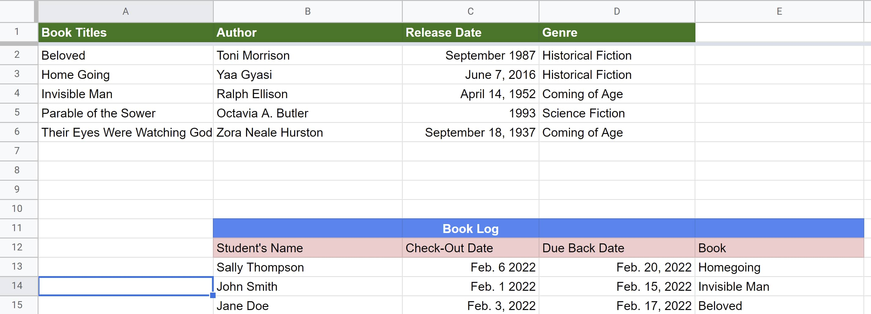
 The example below has two separate graphs on one sheet. Notice the graph containing book titles, authors, release date, etc … is organized by alphabetical order, while the book log below it is not.
That’s because the graph of book titles was sorted by range so it wouldn’t disrupt the book log below it.
How to Sort Columns and Rows in Google Sheets
Knowing how to sort rows and columns in Google Sheets is key to organizing your data. Here’s a step-by-step guide:
Alphabetical or Numerical Order
Step 1: Open a spreadsheet in Google Sheets and highlight the group of cells you’d like to sort. In this example, we’ll use the graph of book titles.
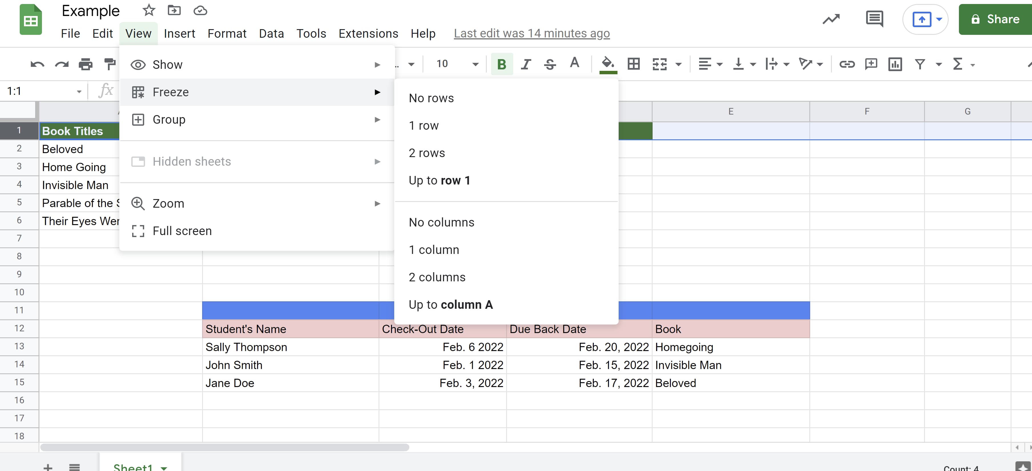
 If your sheet has a header row (like the green header row in the example), you’re going to want to freeze that row so it stays in place as you sort.
To do this, select the header row, click the “View” tab, click “Freeze,” then click “1 row.” If you do not have a header row, then you can move on to the next step.
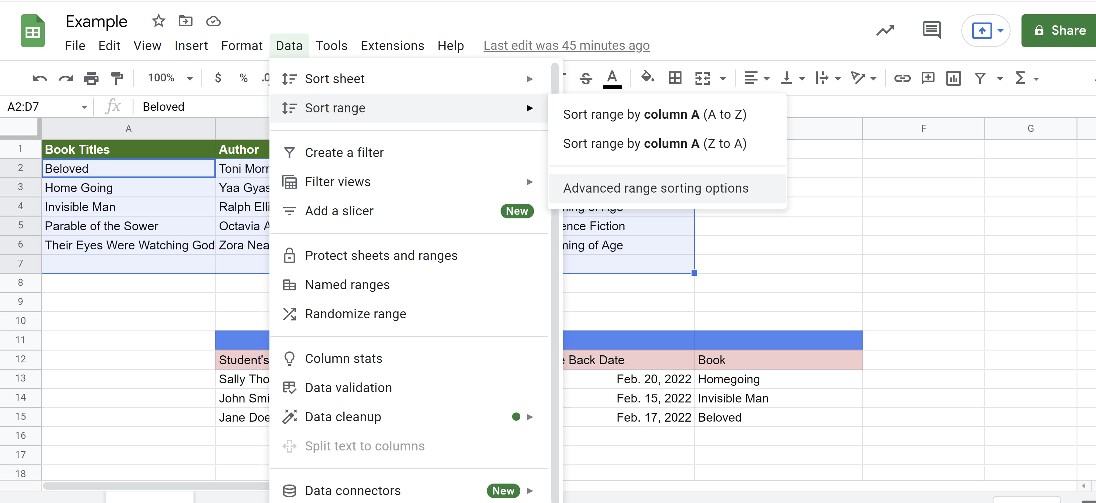
 Step 2: Click the “Data” tab then “Sort Range” then “Advanced range sorting options.”
 Step 3: If your columns have titles, click “Data has header row.”
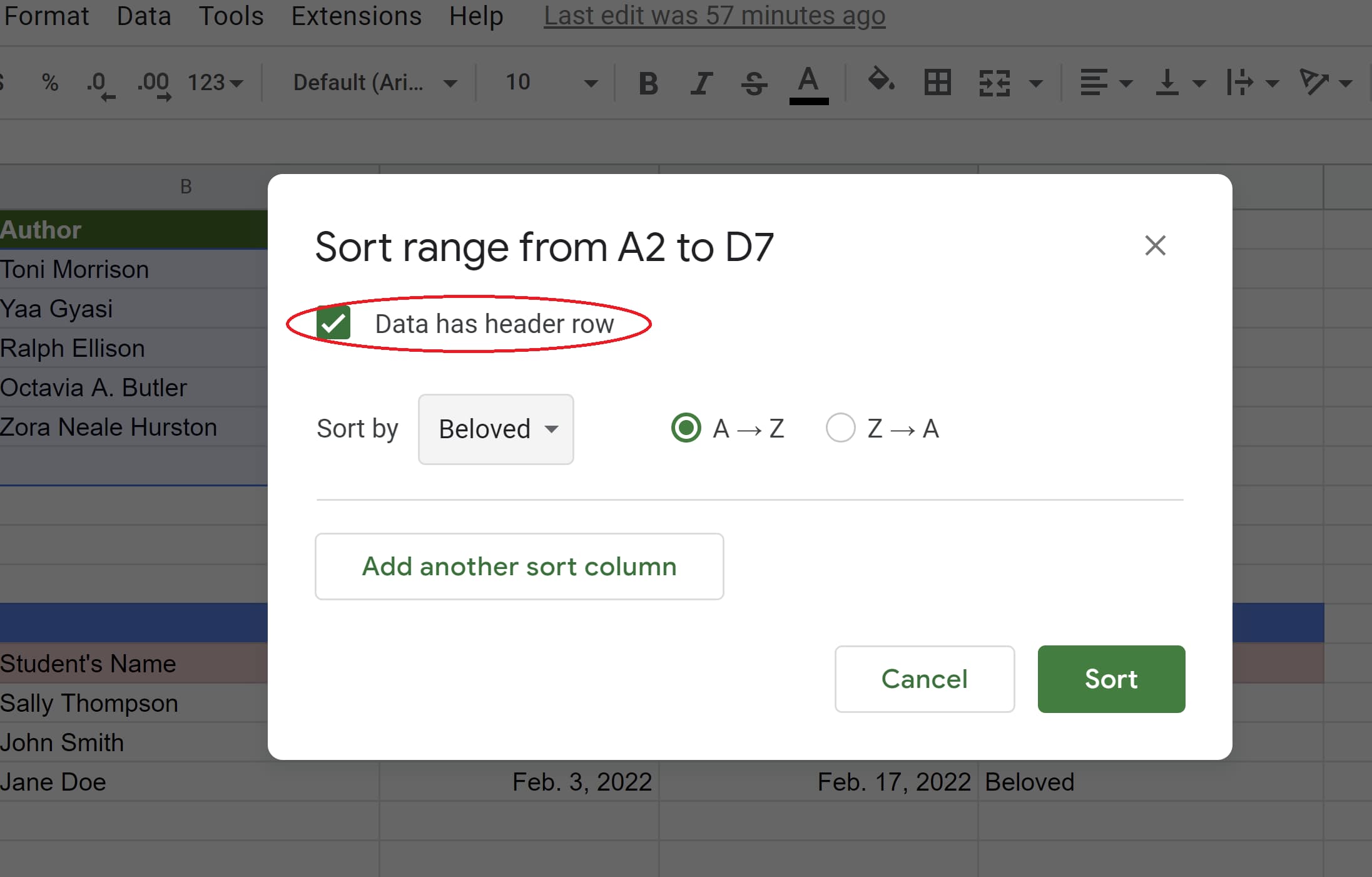 Step 4: Select the column you want to sort first then choose the sorting order. A-Z and Z-A will put your data in alphabetical and reverse alphabetical order respectively.
If you’re working with numbers, A-Z will organize the data in ascending order and Z-A will organize it in descending order.
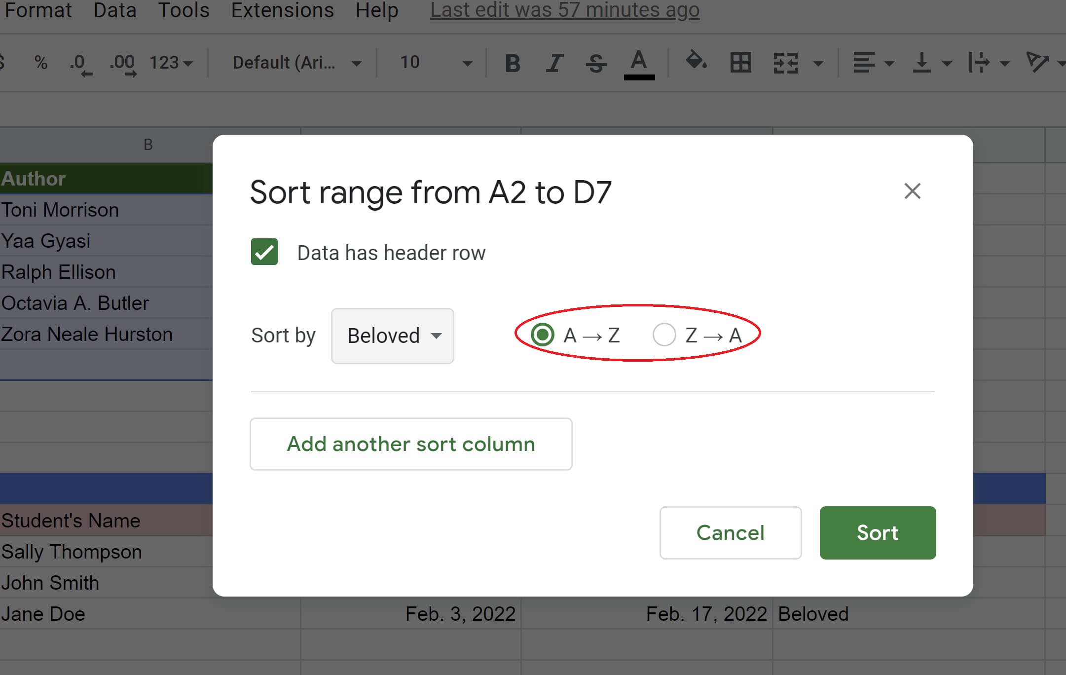
Step 5: To add another sorting rule, click “Add another sort column.” Then click the green “Sort” button.
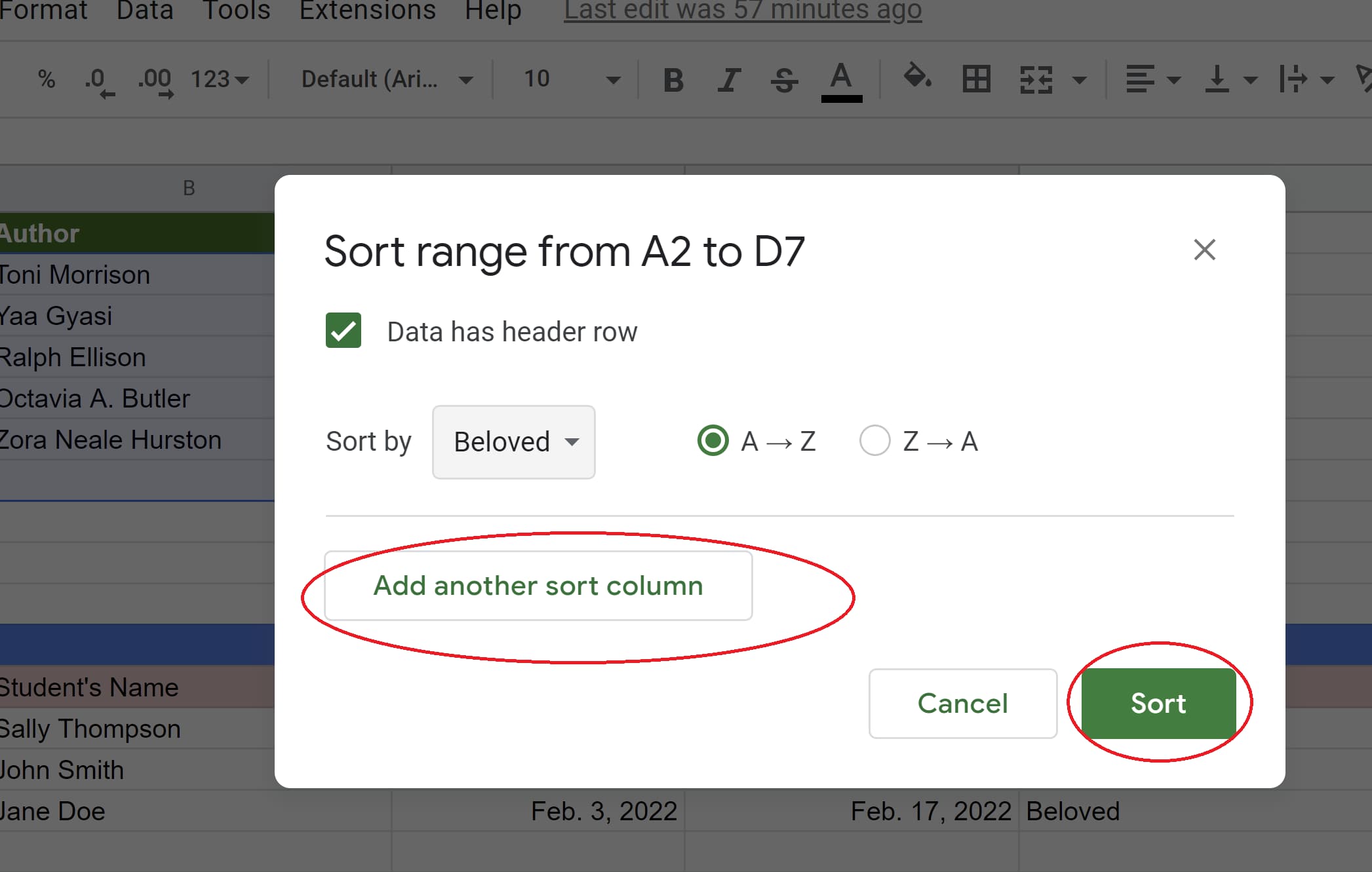 Step 6: To sort an entire sheet, right-click the letter of the column you want to sort by, then click sort A-Z or Z-A.
How to Filter Your Data
Filtering your data is especially helpful if you want to hone in on specific information from a large data set. It’s also great if you only want certain information displayed when people first open your spreadsheet.
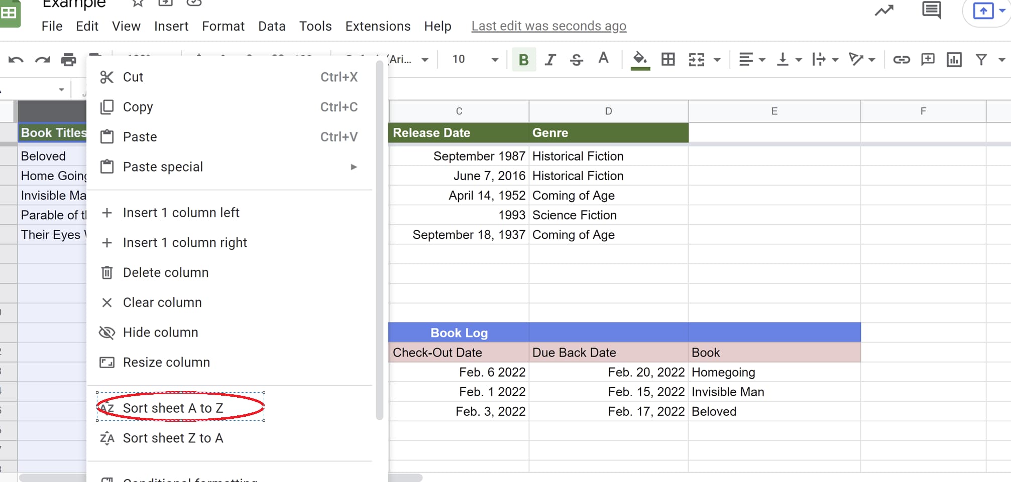
Step 1: Select the range of cells you want to filter.
 Step 2: Click the “Data” tab then click “Create a filter.”
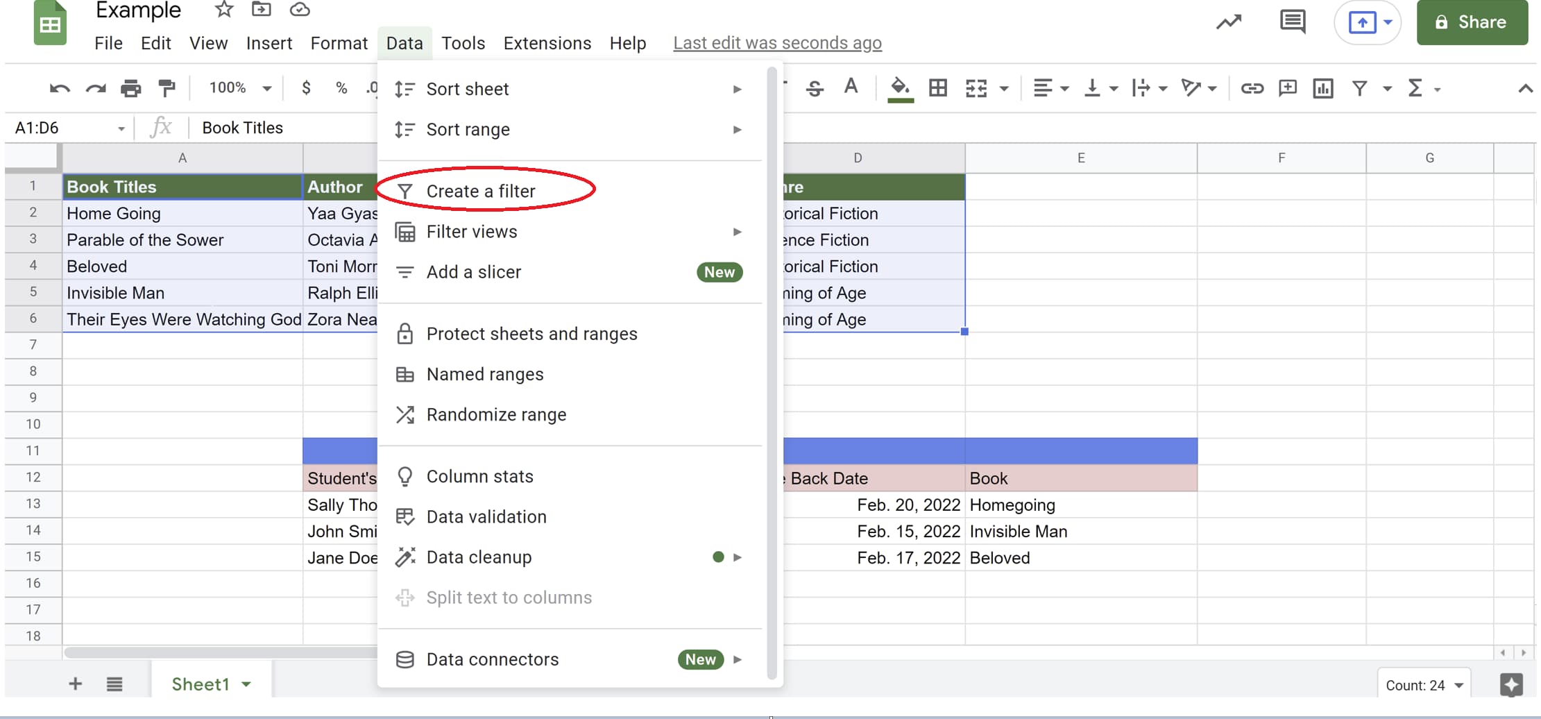 After clicking “Create a filter,” your graph should look like the example below. Notice the filter icons next to each column header name and the new border around the graph.
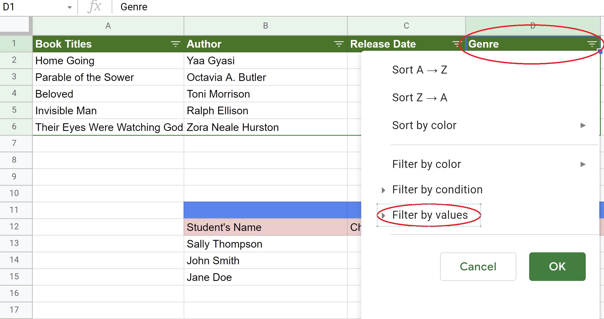
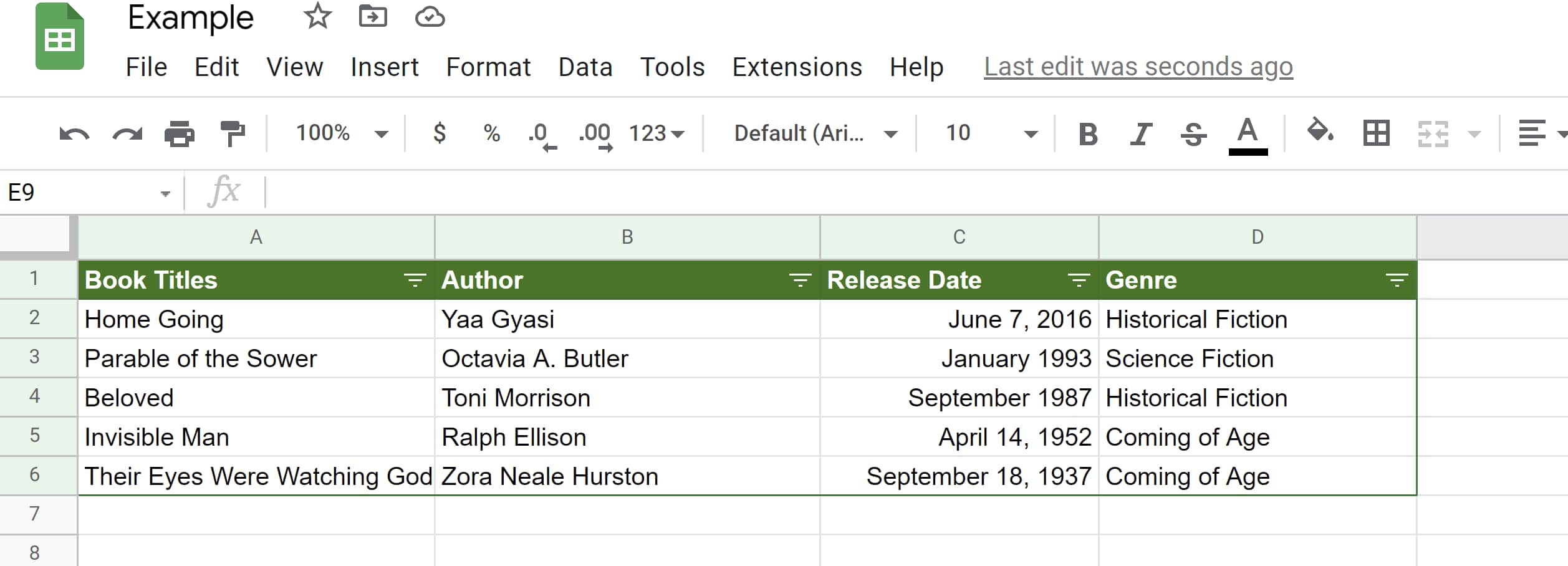 Step 3: Let’s say we only want to see book titles that are historical fiction. To do this, we’d click on the filter icon next to “Genre,” then click “Filter by values.”
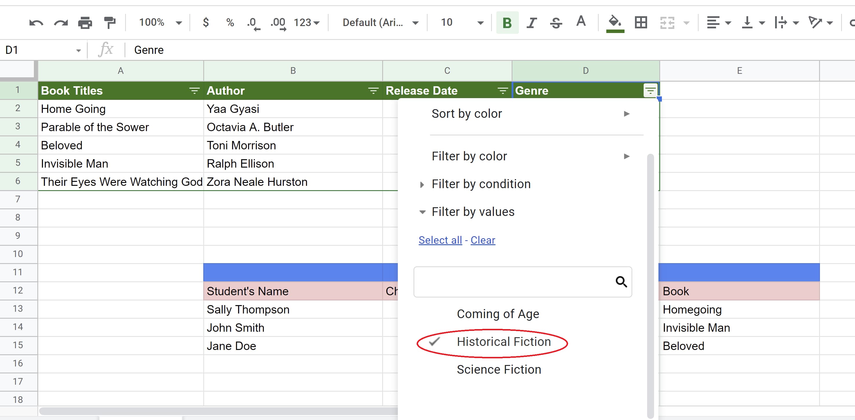
 Step 4: Then, we’d uncheck everything but “Historical Fiction,” and click “OK.”
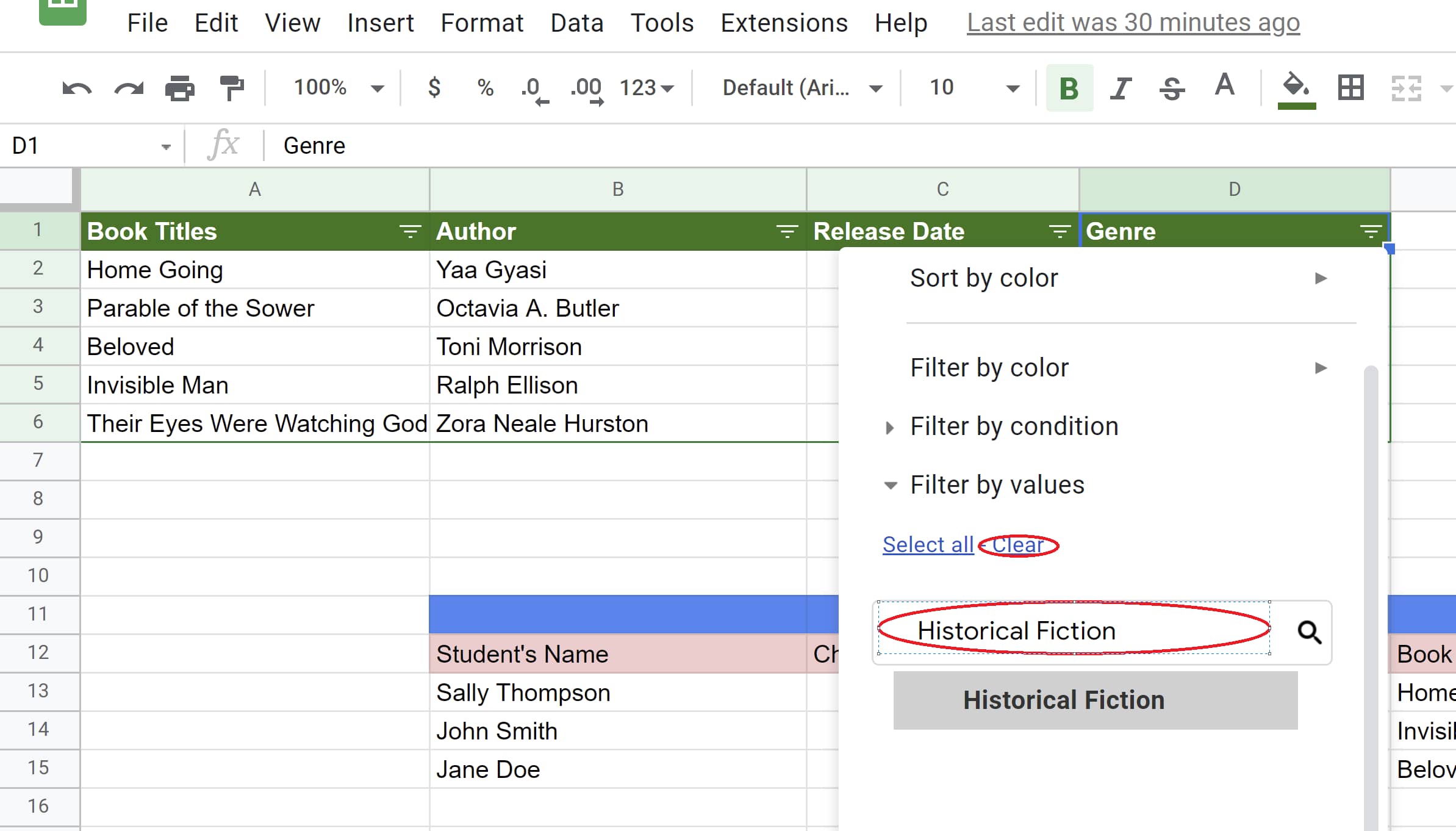
 This can also be done by clicking “Clear” and typing in “Historical Fiction.” The latter method is great if the value you want to sort by isn’t listed and you want to add your own.
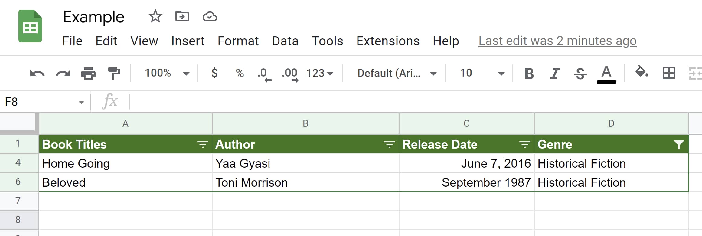
 No matter which method you choose, the end result should look like this:
How to Sort Your Data by Color
Let’s say the book titles are all color-coded by genre with historical fiction being orange, science fiction being blue, and coming of age being purple.
To sort these color-coded titles so that coming-of-age books are at the top, do the following:
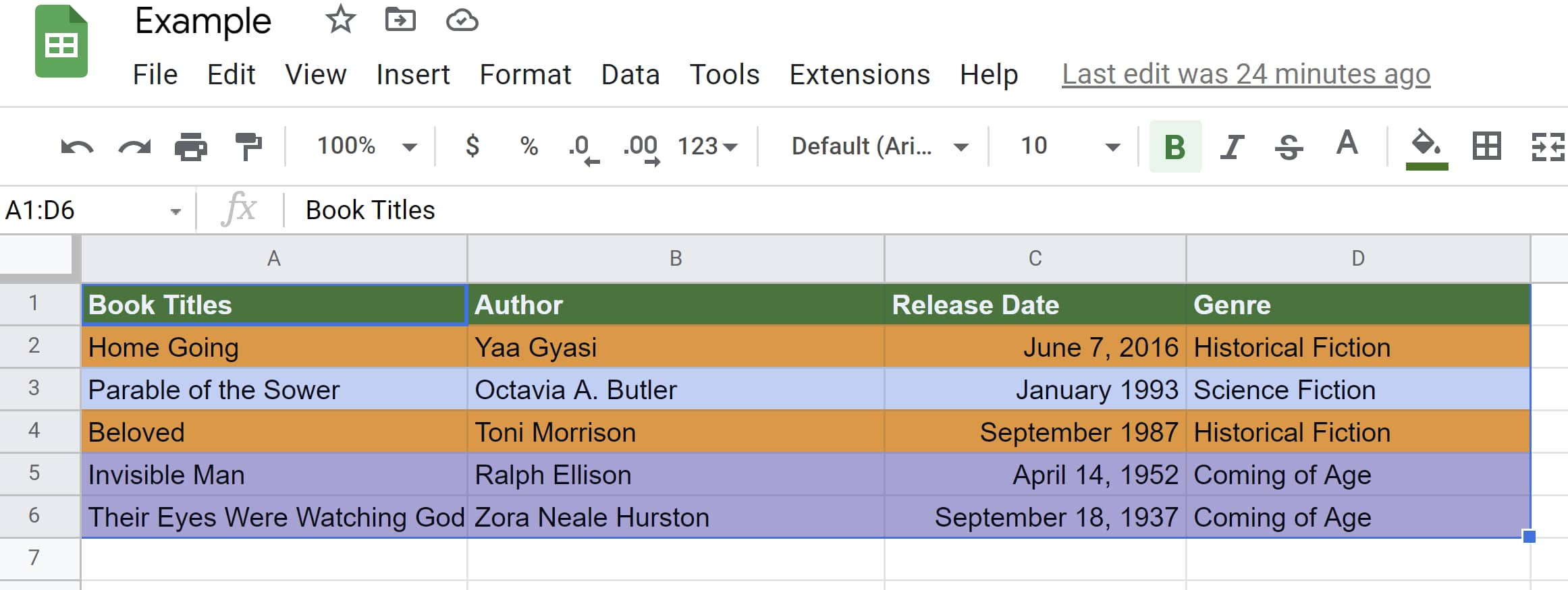
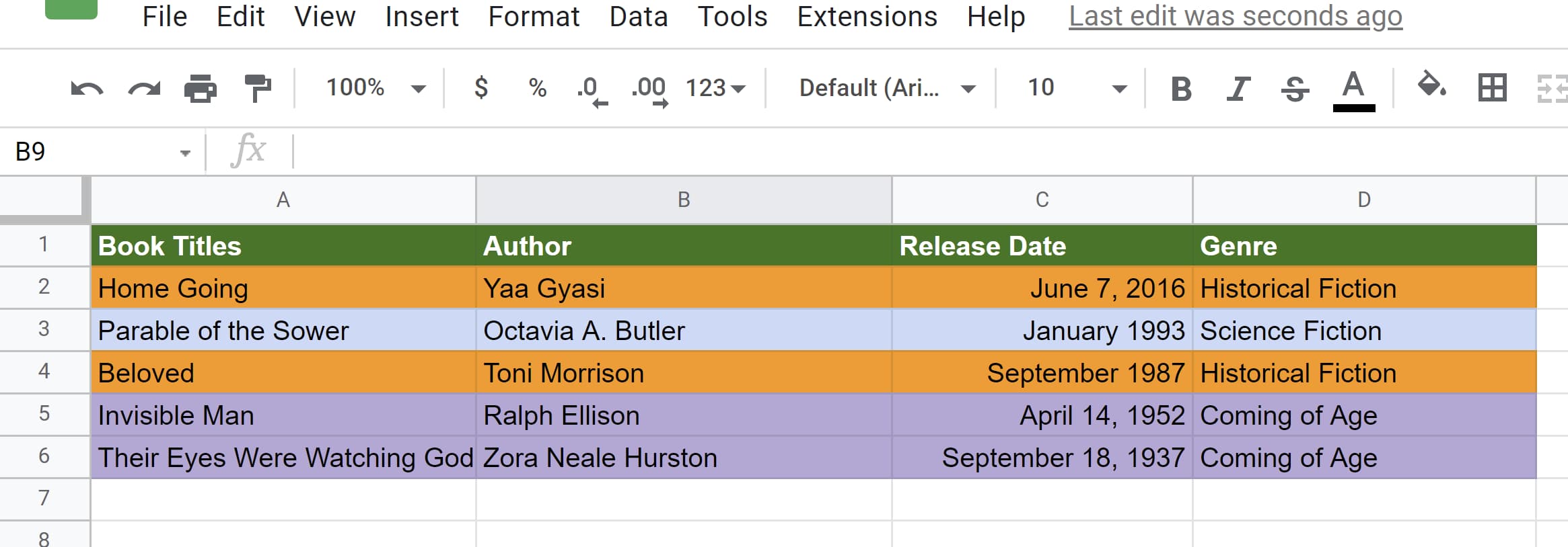 Step 1: Select the range of cells.
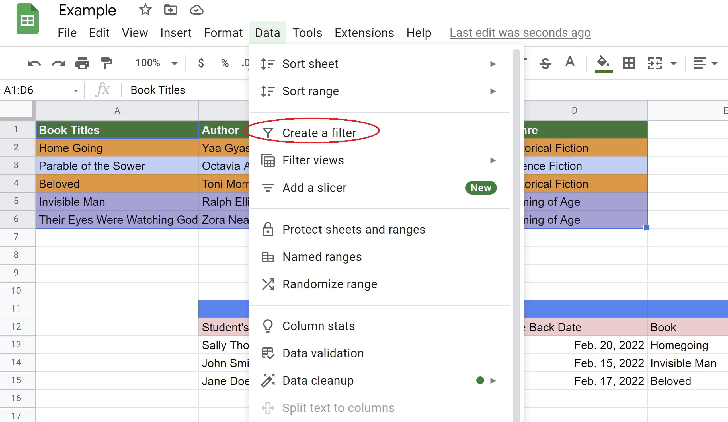
 Step 2: Click the “Data” tab then click “Create a filter.”
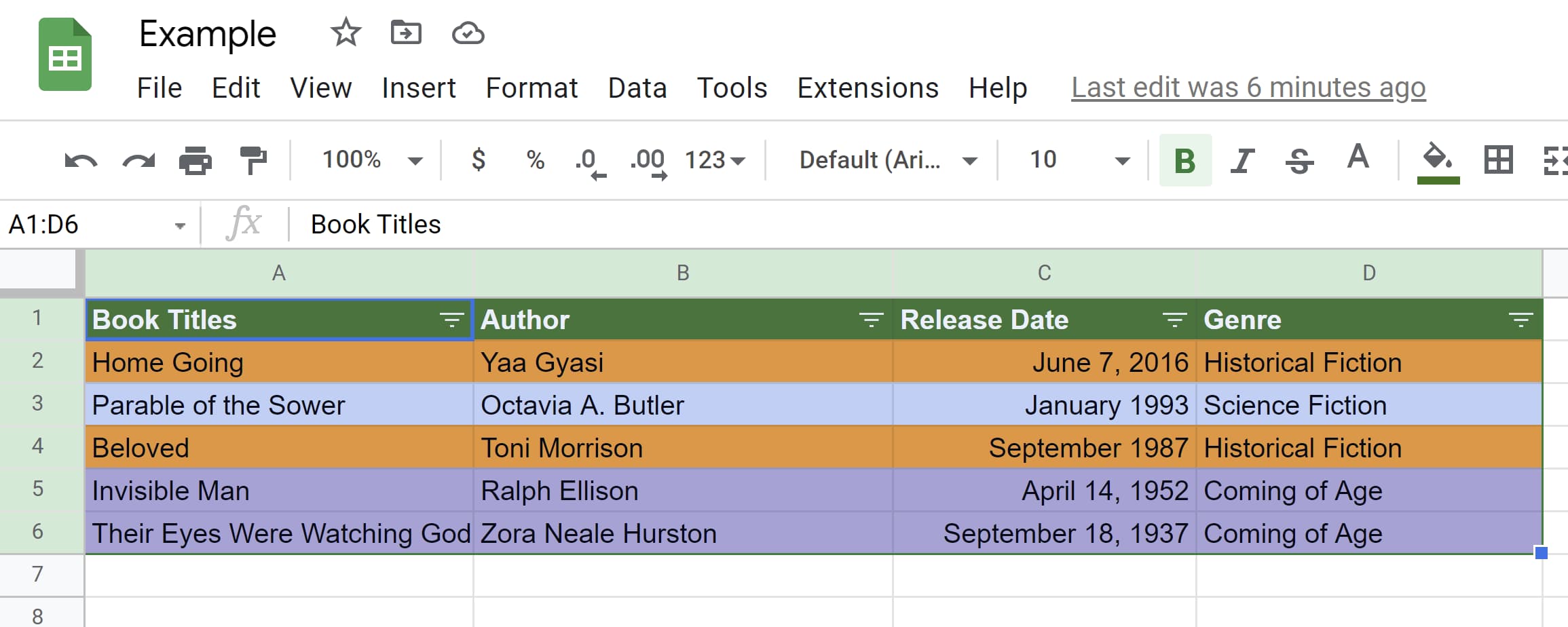 Step 3: Click the filter symbol in the genre column, then sort by color, fill color, then purple.
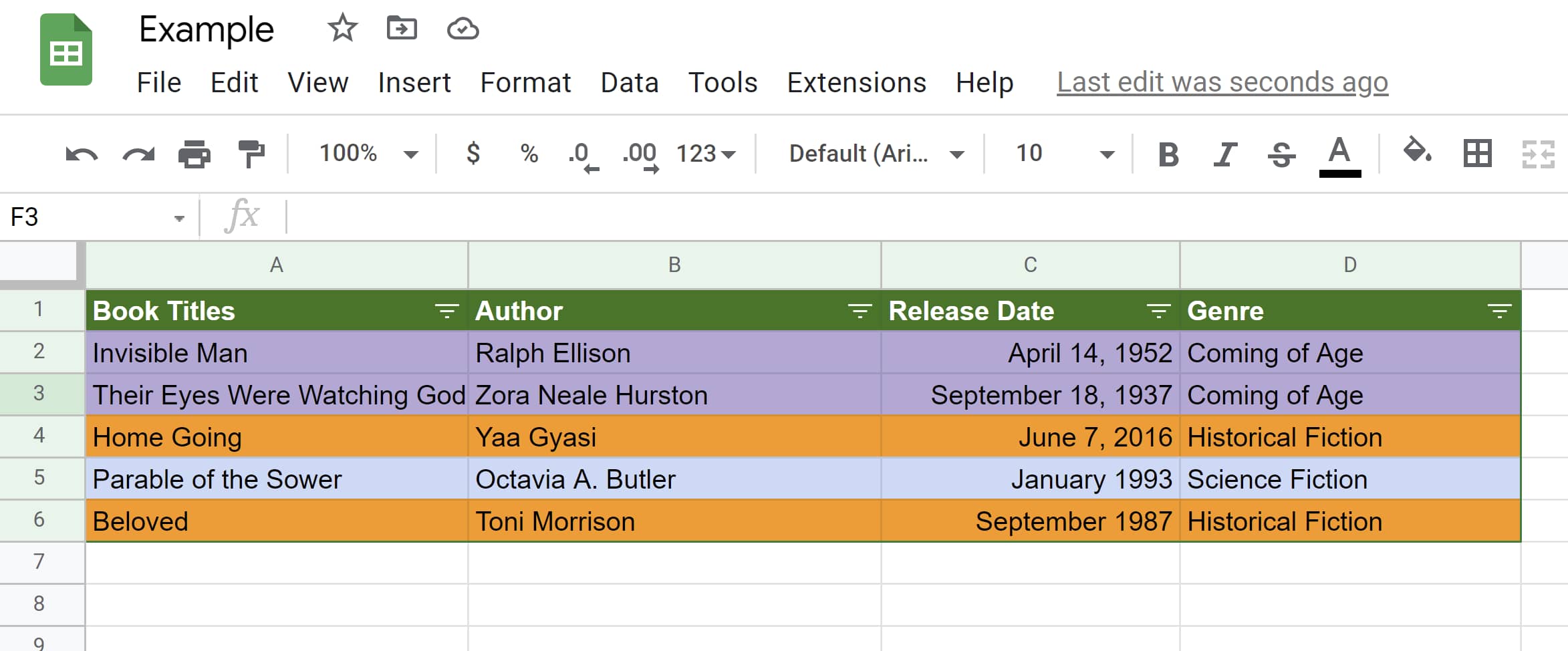
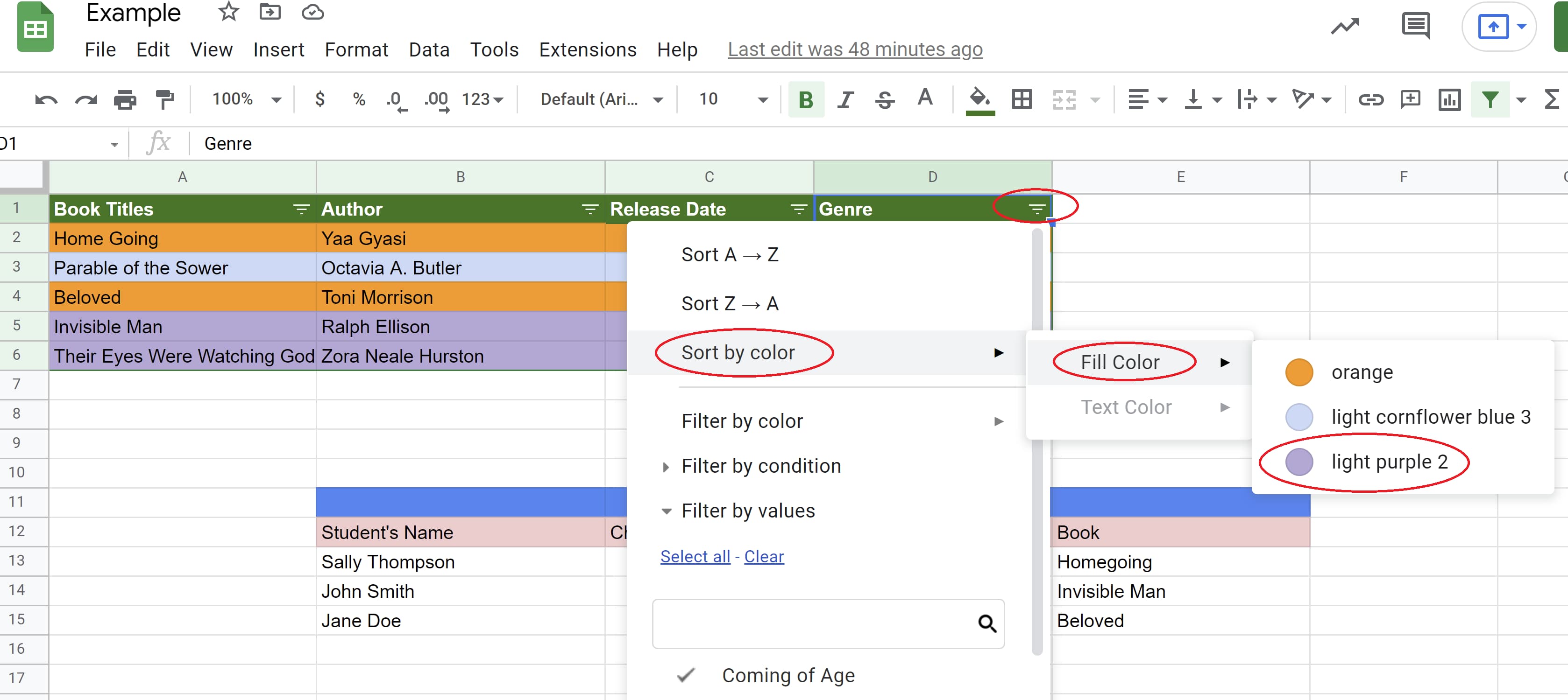 After doing so, all coming-of-age titles will appear at the top of the graph.
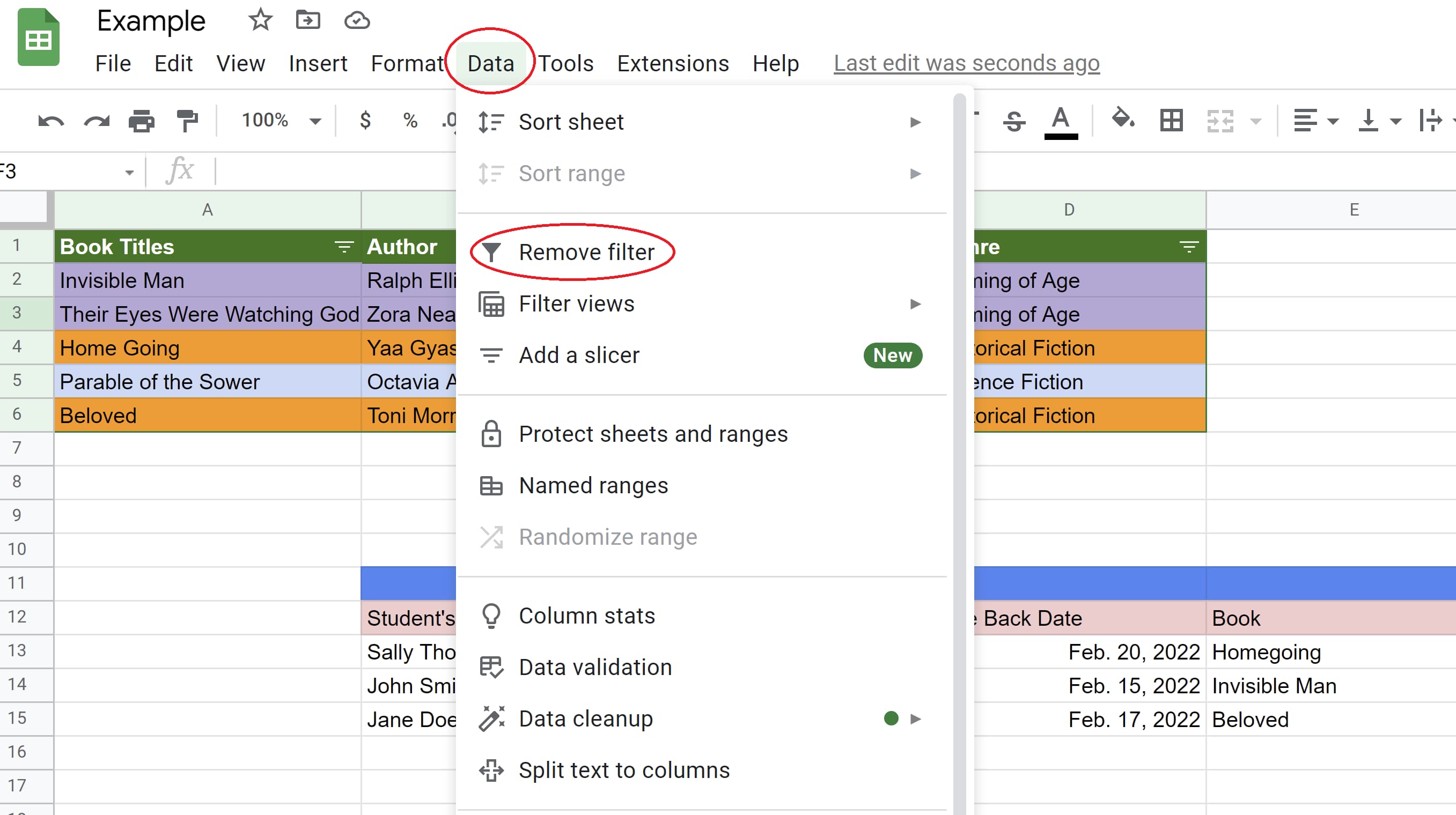
 If you’d like to turn the filter off, simply click “Data” then “Remove filter.”
Remember that your filter will be visible to anyone with access to the spreadsheet. If someone has permission to edit your spreadsheet, that person can also change the filter.
And that’s how you can sort and filter your data in Google Sheets. Now you’ll be able to organize your data digitally in one application.
Remember, Google Sheets is available for free to anyone with a Google account or Google Workspace account. It’s also ideal for collaborative projects thanks to Google’s sharing and editing features. Happy sorting!
![]()

![→ Access Now: Google Sheets Templates [Free Kit]](https://i4lead.com/wp-content/uploads/2022/04/e7cd3f82-cab9-4017-b019-ee3fc550e0b5-1.png)
